Updates February 2021: The AVNA1 User's Manual has been completed and includes detailed instructions as well as background material. The Manual is available for download as a PDF document. This all happened because Evans Wetmore, K3VFA, took all the rough and unorganized notes and turned them into a real manual. Thanks, Evans.
Updates Nov 2020: The AVNA hardware stays the same, but version 0.84 of the software has had major additions of a spectrum analyzer, a vector voltmeter, multiple signal generators, and a Gaussian white noise generator. Added also are calibrations for input/output levels and the touch screen and BMP Screen Save. The software source can now be downloaded as a single package from GitHub.
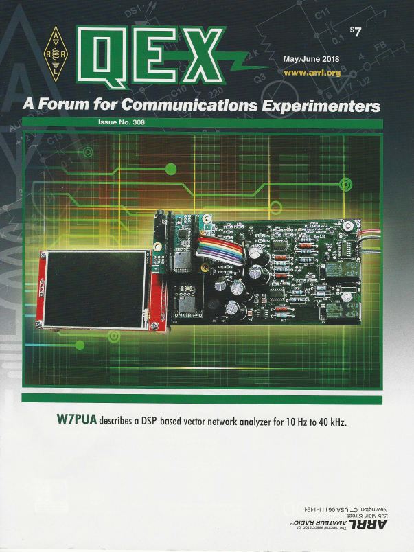
This is the Web page for information on the Audio Vector Network Analyzer project. The article, "DSP-Based Vector Network Analyzer for 10 Hz to 40 KHz" is in QEX magazine for May/June 2018. This is published by the ARRL. Extra files for this project will be available from the ARRL These include source code for the Teensy 3.6, a part list, and Gerber files for the PCB. NOTE: The files referenced in the QEX article are a snapshot of Spring 2017. Improvements made since then are not reflected in those files. Thus the references below, and particularly the control .INO software, reflect the latest updates. The PCB Gerber files at the ARRL are current.
email Discussion Group - A group has been put together to get questions answered and to coordinate part purchases. This is the regular email reflector deal through groups.io. You have the options of "no-emails," "individual emails," or "daily digests." To subscribe, you can either go to groups.io, click "Find or Create a Group," and then search for the group, "AVNA1" or alternatively just use the form at the bottom of this Web page. Information on privacy and other issues is at the groups.io Web site. Be sure to join this group if you want to build this project.
Introduction - First, before getting into the details, let's explore the reasons why the AVNA might belong with your test equipment. For me, it started with using VNA's for years with radio frequency (RF) measurements. Of late, I use the N2PK VNA a lot for 50 KHz to 60 MHz work. This allows impedance measurements of both resistance and reactance. It also allows transmission measurements through a device such as a filter, that show both the frequency amplitude response, but also the phase shift. The phase shift measurements are not always needed, but at time they can be very useful. The most obvious example, perhaps, is to measure a phase shift network that needs to produce, say, a 90 degree shift. Another example would be a feedback amplifier that is stable and/or useful only under certain phase shift conditions.
In a nutshell, all these same needs exist at low frequencies, such as the 10 to 40,000 Hz range of this VNA! This means that components such as inductors and capacitors can be measured accurately, including the internal series resistance of capacitors or the Q of inductors. Components, such as electrolytic capacitors or ferrite-cored inductors that frequency-dependent losses can be characterized. Circuits, such as audio phase shift networks, can be measured for gain and phase shift. This is useful for design, but probably even more so when something needs troubleshooting. Circuits, such as low-drop-out voltage regulators, have requirements on the maximum Q of capacitors that can be measured.
And then, the AVNA is a handy, easy to use tool for just checking components before using in a project. It is a quick and easy way to confirm the value of R-L-C components.
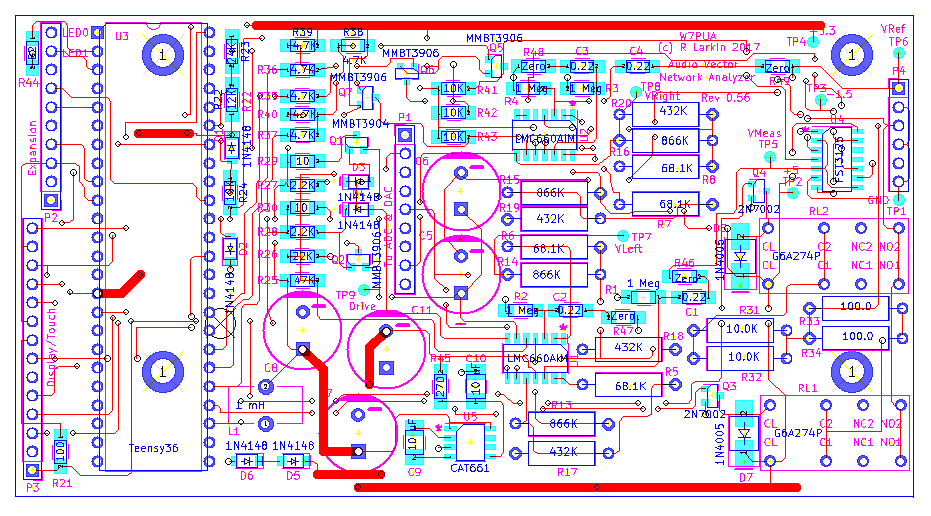
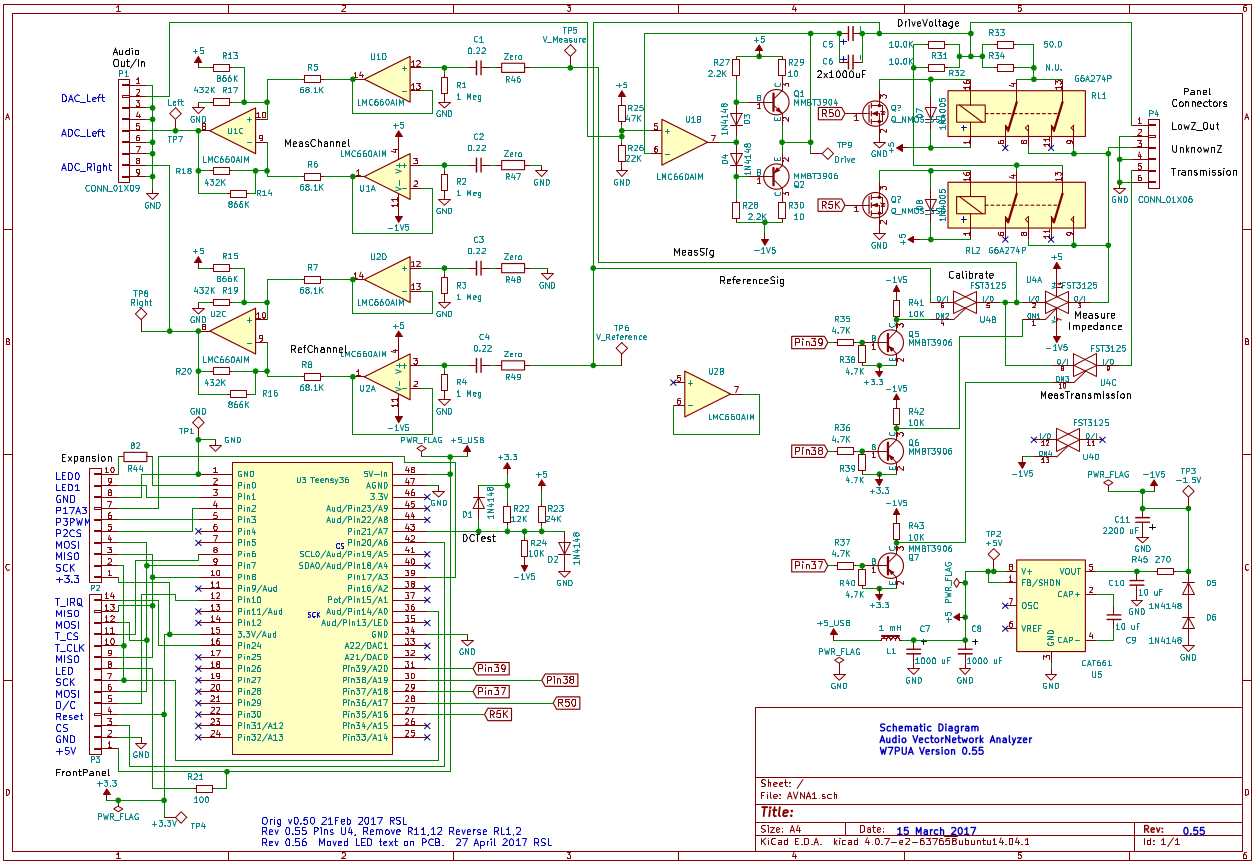
Schematic - Here is the schematic in GIF.
Components - The PC board is produced from Gerber files that are posted in a .ZIP file inside the extra files noted above. You do not need to order boards from Gerbers, as these are already set-up at OSH Park. These "shared project" PC Boards are available in multiples of three from OSH Park. As long as you have two others to also buy boards, this is a very reasonably price source as well as a simple ordering procedure.
The schematic and symbols, in KiCad format (ASCII), are available in the same QEX files. This is a start for a modified PCB if you desire. If you are serious about changing the PC board in KiCad, email me for the PCB files. I am not posting these, as the footprint files are scattered in directories and need organizing.
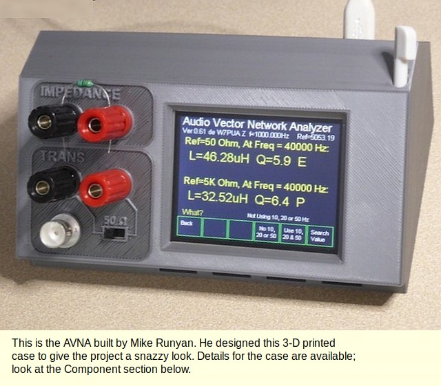
The great looking 3-D Printed Case, seen at the top of the page, was designed and printed by Mike Runyan. Mike has provided the files for the case and a bunch of details and pictures. These are on a separate page linked here.
Part List - The part list at the QEX additional files will be supplemented here as information is available. A version 2 part list is available here. Changes include:
Component matching - The inputs to the ADC's are a pair of instrumentation amplifiers. U1D, U1A and U1C are one of these and U2D, U2A and U2C are the other. Each of these has considerable symmetry that is used to cancel errors. We can help maintain this symmetry by matching resistors. What this involves is buying 10 or 20 resistors when we only need 4. Go through these with a digital ohmmeter and find pairs that are close, ignoring the exact value. If we start with 1% resistors, we can often match them to 0.1%. Pairs to be matched (follow this on the schematic and it will be more clear):
Construction -
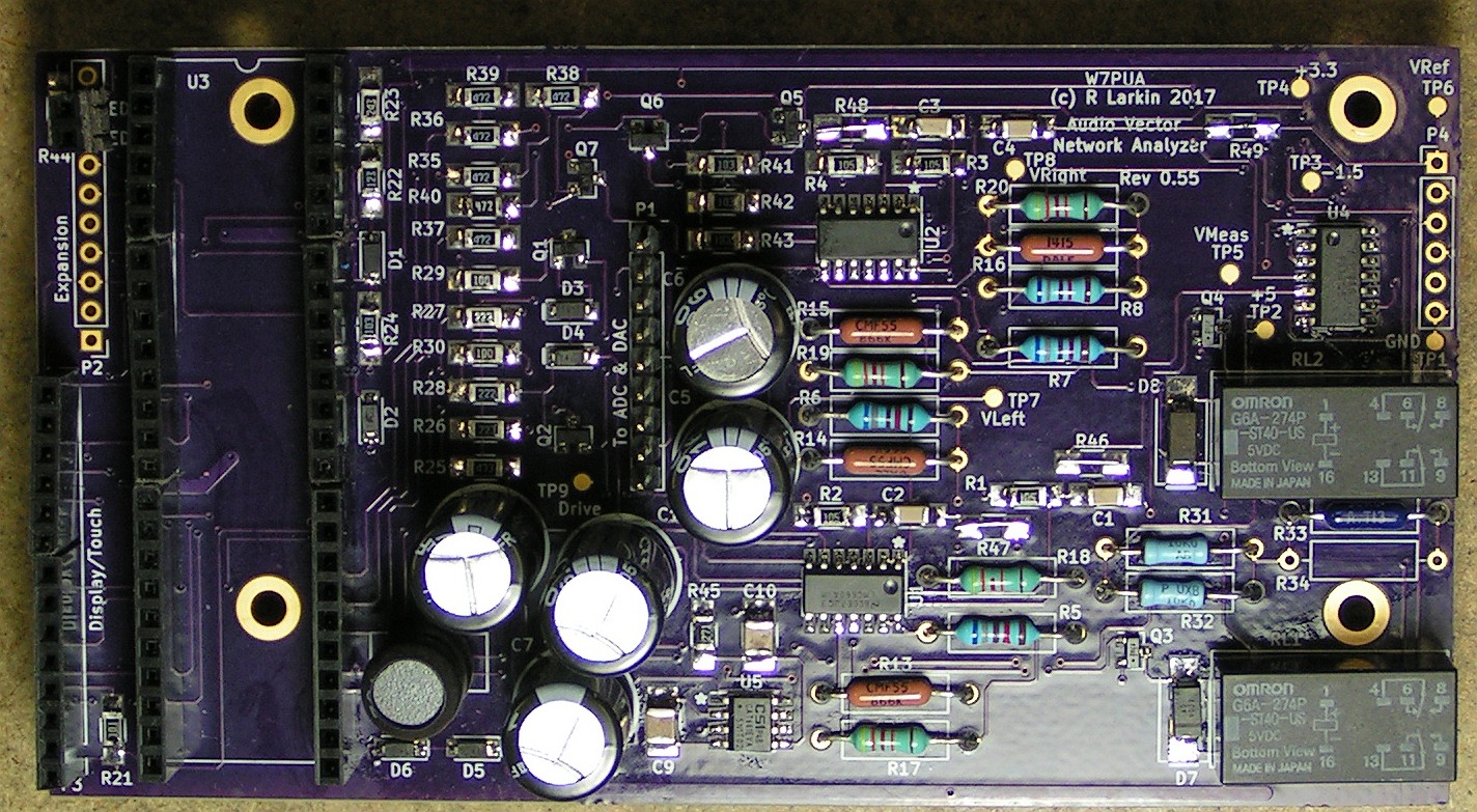
The board is a combination of leaded components a surface mounted parts. We were fortunate to be able to find IC's with relatively large pin spacing of 0.05-inches. Leaded components were used for the precision resistors as that increased the available selection of parts. The Teensy 3.6 board has all of the functions used in the AVNA coming to the 24 pins on each side. The bottom of the Teensy should have 48 header pins poking downwards. But, in addition, the top of the Teensy needs to hold the Audio adaptor board. The easy way to do his is with stackable headers:
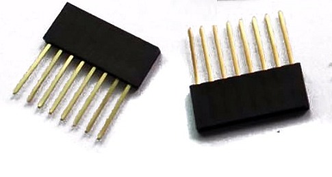 These are stackable headers. You need to have all the pins of the Teensy that mate up with the Audio Adaptor
(2 x 14 pins) use these. It is not much more work is to use these on all 48 Teensy pins. These mount on top of the Teensy board with the pins going down.
You will probably find the longest available stackable headers to be 8 or 10 pins and thus need to position several of these, end-to-end.
This may require some sanding on the ends of the stackable headers.
These are stackable headers. You need to have all the pins of the Teensy that mate up with the Audio Adaptor
(2 x 14 pins) use these. It is not much more work is to use these on all 48 Teensy pins. These mount on top of the Teensy board with the pins going down.
You will probably find the longest available stackable headers to be 8 or 10 pins and thus need to position several of these, end-to-end.
This may require some sanding on the ends of the stackable headers.
Socket P3 (display) requires a 14-pin socket that is on the top of the board. I put header pins on the display and plugged it into this socket. There is greater flexibility in mounting location for the display if wires are arranged between the display and the main board. This can be done in several ways including soldered wires.
Pins 9 and 10 of P2 are for a red/green LED. Again the connection for these two should be wires. P1 is 9-pins and connects by wires to the audio I/O of the Audio Adapter board.
Assembly of the PCB should start with low components to avoid hitting taller ones with a soldering iron. The part list can be used to keep track of parts that have been installed. The electrolytic capacitors
The enclosure need to be solid for mounting the parts being tested. It does not need full shielding, but that would not hurt. Check carefully for the mounting position of the display, watching for where the connecting wires will go. I chose to make the enclosure from plywood, as I had a shop that made that easy. I placed copper adhesive tape around the bottom and edges to provide common ground connections.

Checkout and Testing - The powering of the AVNA is complete when a USB "micro-B" cable is attached to the Teensy board. This provides +5 Volts to the main board (mine measured 4.68 Volts at TP2). At that point, the negative 1.5 Volt converter can be measured (mine measured -1.36 Volts at TP3). The display board should be back-lighted, but no data will show. The LED is probably off. Not much happens until a program is installed.
Program installation requires several steps. These can be done using almost any PC. My only experience is with an Arduino IDE running under Linux. What I have here may differ in detail for other operating systems. The following is for a full INO compile. You probably will want to work at this level eventually, to allow experimentation, but a HEX file load is outlined below that is simpler for some.
Starting with version 0.60, a configuration file is required. As of now, this file allows the orientation of the display and touch screens to be set individually. Edit this file to suit the individual screen. The configuration file for "1 1" orientation is: AVNA1Config.h
NEW with Version 0.80! Software package now at GitHub, all in one package. The Github site https://github.com/boblark/AudioTestInstrument now includes all files for compilation and running the instrument. This includes the external library files files. By following the instructions on the Readme.md file (scroll down on the Github page to read that file without downloading). all files will be placed in the proper directories for the Arduino IDE to find them. You still compile the Teensy program as before. Alternatively, if you do not want to compile this, a file AVNA8main-82.hex (82 or higher) is ready to be loaded using the PJRC Teensyduino loader. The .hex file is a standard Intel hex image file. This simplifies the installation of new software considerably.
Hex file software images - Also, starting with Version 0.82, Intel Hex Teensy 3.6 image files are at the GitHub site. These are in a "hex" folder with names like AVNA8main-82.hex. These are the hex files that the Teensy Loader works with. If you compile the AVNA software in a standard model (Arduino IDE + Teensyduino add-on), you do not need these files. You automatically generate them, and the Teensy Loader automatically uses them. The hex files are on GitHub in case you are having problems with the compilation process and can skip to the loading process.
Previous Teensy .INO Control Software - Several previous versions are available here. These pre-date the dividing of the INO into sections and control of this under Github. Click here
    RSL_VNA5.ino      Ver 0.61 1 Nov 2018
    RSL_VNA5_60.ino   Ver 0.60 2 June 2018
    RSL_VNA5_59.ino   Ver 0.59 29 May 2018
    RSL_VNA5_58.ino   Ver 0.58 23 May 2018
Versions 0.59 through 0.80 require the latest XPT2046_Touchscreen.h and .cpp in the Arduino libraries. These are available from gitHub. Installation info is at Arduino. See the section on using the library Zip file. UPDATE: Starting with Version 0.81, the GitHub ZIP download includes all external libraries.
The AVNA1 User's Manual is now available and is the main source of information on operating the unit. It includes screen shots and detailed instructions as well as technical background on the measurements. The Serial Command information has been enlarged and included in the manual.
Tuneup calibration of the AVNA (UPDATE: See the notes at the bottom of this page for additional Cal information on Input, Output and Touch Screen calibrations.) For impedance measurement with the AVNA, the word "Calibration" has meant two different things, (1) the adjustment of amplitude and phase between the reference and measurement channels (the CAL or C command) and (2) the selection of input circuit components to maximize the accuracy (TUNEUP command or manual PARAM1 and PARAM2 changes). I am going to try to use the word "tuneup" to refer only to the second usage to minimize confusion. So, it is this (2)-type "tuneup" that we are addressing here.
Most of the tuneup of the AVNA resides with determining the value of the precision 50 and 5000 Ohm resistors inside the unit. But, there is more that can be done to compensate for "stray" impedances, including the wiring capacity. Beginning with version 0.61 we have two alternative methods for setting the six component values. The old method was to measure the 50 and 5000 Ohm resistors and then try different values for the other four and see what worked best. The details for this are in the Direct Tuneup notes. The new approach carefully measures the input impedance with short, 50-Ohm, 5000-Ohm and open terminations. From this the six values are directly calculated. Good details on this method are in the Indirect Tuneup notes.
Which method is better is an open question. For a start, I would suggest the second indirect method, as it moves directly to answers and if things go well, it does not take long. Keep in mind that the two methods can be combined, since the values can be entered manually. It is probably good for learning to try both methods, keeping notes as you go.
Serial Control - The AVNA1 is fully controllable by a serial link. This physically is the USB cable connecting the AVNA to a host PC/laptop. The various commands are detailed in Section 12 of AVNA1 User's Manual which replaces the Serial Command document.
Screen shots can be taken either to an internal microSD card or to the Serial link. This again is fully covered in the User's Manual.
Battery Operation - Probably the most universal way to power the AVNA is a USB battery pack. Here is one, but they are available everywhere in different sizes and quality. The AVNA draws about 200 mA and so if you avoid "just leaving it on," a charge lasts months. It takes about 3-seconds to load and run the program at start-up, so turning it off when it is not being used is not an issue.
Note - With the 0.80 revision comes many new functions, such as a spectrum analyzer and multiple signal generators. No detailed measurements are shown here, but the User's manual does includes some simple examples of the new instrument use, as well as details of the controls.
Additional AVNA Measurements - The QEX article has some data measured with the AVNA. Here are a few more that might be of interest.
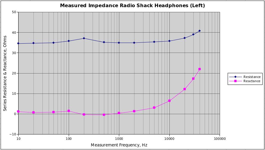
This first measurement is a set of headphones that have been around for probably 10 years. All they say on them is "Radio Shack."
Nothing about models or impedance is on them. So just for fun and education, I measured the impedance of the left unit using
the 50-Ohm reference in the AVNA:
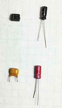
Update, 9 Oct 2018 - Tantalum capacitor replacement - My 1984 vintage Tek 494AP Spectrum Analyzer is developing a phase noise problem. I thought that it might be caused by the old tantalum capacitors that are used throughout the instrument for bypassing and filtering. The usual approach to this type of problem is to replace the capacitors and see if the problem is fixed. I thought the AVNA might allow a more sophisticated approach by measuring the old caps, along with the proposed replacements. Many of the capacitors involved were 10 uF at 20 Volt surface mount tantalums, as shown in the upper left of the photo. Over the years, electrolytic capacitors have improved in performance as well as size efficiency. Thus, the intended replacement was a leaded 10 uF 63 Volt. A leaded type was chosen since current surface mount types are too small to fit the pad pattern of the Analyzer. This was updated 8 Oct 2018 to show the impedance of "New" tantalum capacitors.
Here are details of setting up the AVNA to measure the parts with the control all from the Serial Monitor in the Arduino IDE. The AVNA was connected to the PC USB port and the Arduino IDE was opened. The Serial Monitor (terminal) was selected from the Tools menu. If you have problems at this point, it probably relates to the selection of Menu/Tools/Port. The details vary with operating system, but under Linux I select the port named, "dev/ttyACM0(Teensy)". With the serial port working, the AVNA was setup for swept impedance measurements by sending the "ZMEAS 50", "SWEEP" and "CAL" commands from the Arduino Serial Monitor. The data sent to the PC is human readable, and for this use we will turn that feature off with a pair of commands, "VERBOSE 0" and "ANNOTATE 0". We still get two lines per measurement, one for a series R-X model and the other for the alternate description of a parallel G-B. We only need the first of these, so we issue the command, "SERPAR 1 0". From here, every time we give a "RUN 1" command, we get a set of 13 measurement lines back, corresponding to the standard swept measurement.
The 10 uF tantalum was connected to the Z terminals of the AVNA and the "R 1" command was issued. The 13 lines of data arrived in a few seconds. These were highlighted in the Serial Monitor window and copied to the clipboard with a Ctrl-C. I then opened up a spread sheet program, in my case gnumeric, but any will do. The data was pasted into the sheet involving 5 columns, B through F. Two more columns were added with G being a repeat of B for convenience in graphing, and H being the magnitude of the impedance that was measured. This can all be seen in the following figure.
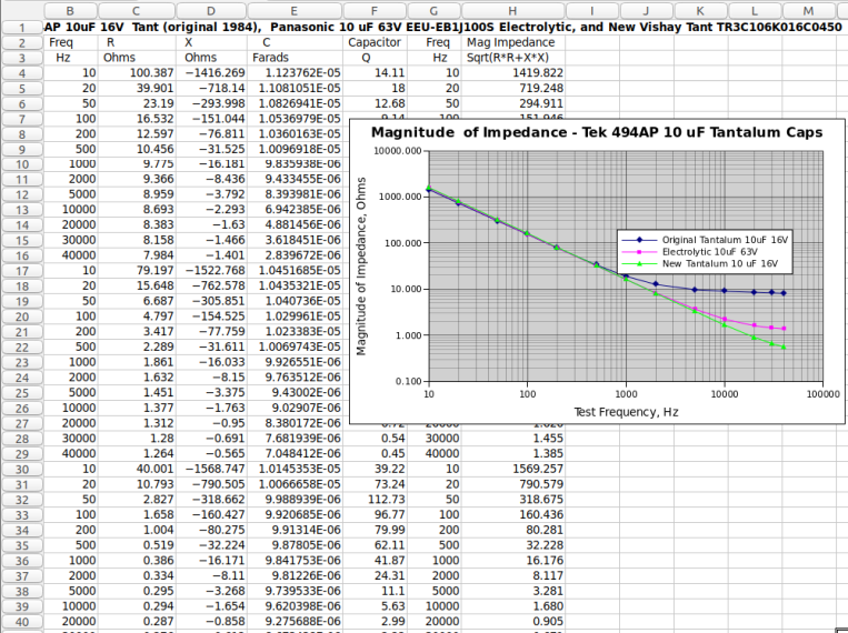
Using the 13 data points a graph was drawn of the impedance magnitude, which is the quantity that determines the quality of a shunt-to-ground bypass capacitor. The x and y axes were both made logarithmic to better show the data. This produced the dark blue trace. This same process was repeated for the new electrolytic, which is shown in magenta. The resulting graph shows that at high frequencies, the impedance is much lower for the new electrolytic. This is due to the drop in series resistance from about 8 Ohms for the tantalum to 1.3 Ohms for electrolytic at the high frequencies. One can suspect that the tantalum is suffering from aging. But, whatever the reason, we have determined that the substitution is unlikely to cause difficulty and probably will be an improvement. An additional note is that the series resistance does vary with frequency, and the measured values can be seen in column C. Above a few thousand Hz, the value is quite constant and this value is the limiting factor for this frequency range. This resistance is also the limiting lower level for the impedance magnitude that is plotted.
The next capacitor was a 47 uF, which is a leaded type. The measurements and graph were created in the same way. Interestingly, the conclusions are different, in that the two impedance curves are almost identical. I would not expect much improvement by changing the types. This simple study gives a good measure as to the improvement expected by changing the capacitors, but does not tell us how the tantalums might have changed over the years. In the case of the 47 uF, maybe the tantalums were better when new.
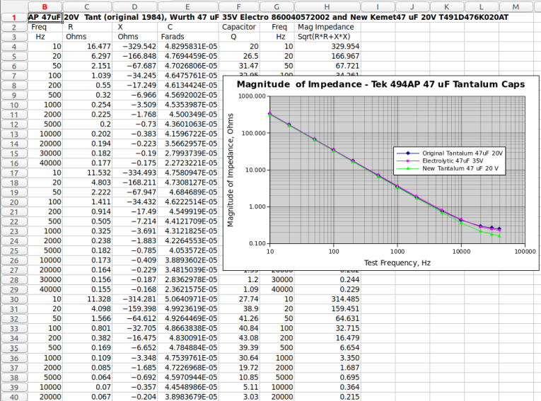
Update 9 Oct 2018 - The original write-up covered the 1984 tantalum capacitors and the new electrolytic equivalents. These are shown in the dark blue and magenta curves, above. This begged for measurements of new tantalum capacitors, and so these were acquired from Mouser. The revised two spread sheet pages, above, show a third green curve for the new tantalums of both 10 uF and 47 uF value. Especially for the 10 uF case, the new tantalums had much lower series resistance (ESR). If this parameter is important, the extra cost is justified. We still do not know if the original tantalums have aged (probably) or were never as good as the new ones. My revised plan for now is to use the tantalums for replacements, in most cases.
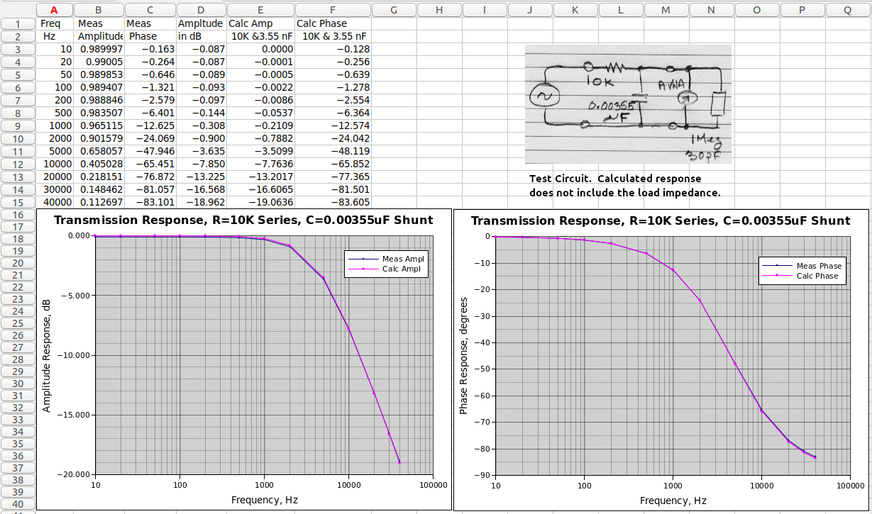
NEW: RC Filter transmission measurement - Here is a sample of a wide-band transmission measurement. The circuit is about as simple as they get, making it easy to compute the expected results. It consists of a series 10K Ohm resistor followed by a shunt capacitor. The capacitor value is marked as 0.0033 uF, but we measured the value as 0.00355 uF, around 5000 Hz, using the AVNA in the impedance mode.
Before measuring this circuit, let's digress to look at several ways that transmission measurements can be made. We are operating in the frequency range of 10 to 40,000 Hz. This gives us the luxury of being able to ignore some of the stray capacities and couplings that make higher frequency measurements more difficult. For instance, at RF frequencies, measurements will be made using coaxial connectors and a standard impedance level, such as 50 Ohms. This has a number of advantages and the AVNA can carry this type of measurement down to 10 Hz with built-in impedance levels of 50 or 5000 Ohms. In addition, low frequency measurements are often made with a true voltage source, corresponding to a zero Ohm impedance level along with an infinite impedance voltmeter that does not load the circuit being tested at all. The AVNA is able to approximate these conditions with a voltage source impedance of less than an Ohm and a measurement voltmeter input of 1-megOhm paralleled with about 30 pF. This configuration is well suited to the RC network described above, and will be used for this measurement.
The low impedance output comes to pin 1 of P4 (ground is pin2) and is independent of whether 50 or 5000 Ohms is selected. The high impedance input goes to pin 5 (ground to pin 6) of P4. These are connections that normally come to the front panel.
Now to the measurements, which can be done manually from the touch screen, or as we will do here, controlled via the Arduino Serial Monitor. The advantage of controlling from the PC is that the output data is easily copied-and-pasted to a spread sheet for analysis. So, the setup commands are "ANNOTATE 0" to stop descriptors, "VERBOSE 0" to stop data that is not directly related, "LINLOG 2 1" to output transmission data as voltage magnitude and phase, TRANSMISSION 50" to set basic measurement, and SWEEP to setup the 13 broad-band frequencies. The calibration for transmission requires that a path be connected between the generator and the load side. For our case, we place a wire between the generator and the load (without the RC network) and issue the command, "CAL".
Next, we put the RC network in place, as shown on the diagram below. The command, "RUN 1" does a single sweep and, in my case, the following data was received by the Serial Monitor:
10.000,0.989997,-0.163
20.000,0.990050,-0.264
50.000,0.989853,-0.646
100.000,0.989407,-1.321
200.000,0.988846,-2.579
500.000,0.983507,-6.401
1000.000,0.965115,-12.625
2000.000,0.901579,-24.069
5000.000,0.658057,-47.946
10000.000,0.405028,-65.451
20000.000,0.218151,-76.872
30000.000,0.148462,-81.057
40000.000,0.112697,-83.101
Each line is a frequency, the voltage received divided by the calibration level and the voltage phase, subtracted from the calibration phase. These are separated by commas, which are recognized as separators by most spread sheets.
The data was pasted into a spread sheet (again, I used gnumeric, but Excel should be fine) and the graphs shown below were created. Two columns were added to calculate the same quantities that were measured, and graphs of these were added. It can be seen that the calculated and measured values agree quite well. One place where they differ slightly is the amplitude at low frequencies, like 10 or 20 Hz. This is due to the 1 Megohm input impedance on the load side. We ignored this during the calculation, but at low frequencies we are left with a 10K series resistor and a 1 Megohm shunt resistor, producing a voltage ratio of (1,000,000 / (1,000,000 + 10,000)) = 0.990099. The measured values were right on at 0.989997 for 10 Hz and 0.99005 for 20 Hz, showing excellent agreement.
You can't see the formulas for the spread sheet, but the calculated ampiitude and phase formulas are (for the 10 Hz line):
Cell E3  "=-10*log10(1+(2*pi()*A3*3.55e-05)^2)"
Cell F3  "=-180*atan(3.55e-05*2*pi()*A3)/pi()"
Issued 21 April, 2018. Last Revised: 7 Feb 2021 - All Copyright © Robert Larkin 2018-2021