A 5.4 to 5.6 MHz 3-Resonator, 0.25 dB Ripple, 50 Ohm Band Pass Filter

We had fine things to say for the direct transformation of the low pass prototype into a band pass filter (See the 9.7 to 14.6 MHz filter) Indeed, that topology is very good for moderate or wide band filters. However, when the percentage bandwidth of the filter gets small, the component values for both the series and shunt elements can become very small or very large. An alternate topology is to have multiple parallel tuned circuits that are coupled on the ungrounded ends (the tops) by capacitors. This opens up a new degree of freedom which is the inductor value(s) for the tuned circuits. More importantly, it allows component values to be adjusted, and for narrow band filters, up to perhaps 10%, it often ends up with more achievable component values.

The transforming of low pass prototypes into this top-coupled topology was formalized by Seymour Cohn in 1957 (see reference 4 on the the main LCFIL3A.BAS page). The referenced paper covers a variety of other implementations of direct coupled filters, as well.

But, getting back on topic, we will move to designing an example top-coupled filter. The example chosen is a three resonator filter with a pass band extending from 5.4 to 5.5 MHz. This might be used along with a crystal filter at 5.5 MHz, either to add far out selectivity, or perhaps to provide a wide band I-F response by itself. The design printout for the top-coupled filter, from LCFIL3A.BAS is:

The component values for the top-coupled filter are at the bottom of the printout. See the low pass filter description for assistance with the exponential notation of part values.

The schematic show all of the component values:

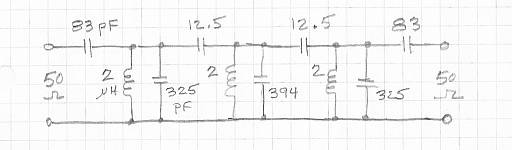
Not shown on the schematic is the impedance level, which from the design print out we see is 50 Ohms. We can simulate the overall response:

This plot shows the insertion loss in a 50-Ohm system as the red curve, MS21 or "magnitude of S21>" It also shows in blue the magnitude of the reflected wave, MS11. This latter quantity, shown in dB is a measure of the impedance match looking into one port of the filter with the other port terminated in 50 Ohms. The curves correspond to lossless components. It can be seen that the 0.25 dB ripple response produces a worst case reflection of about -13 dB. It is difficult to see in the plot, but the ripple dips are 0.25 dB, and these occur at the frequencies of highest MS11.

The top-coupled filter has some interesting characteristics. Note that the response above the pass band does not attenuate as fast as that below the pass band. The top coupling capacitors, of course, are creating this asymmetry. In addition, if you go far above the pass band, the attenuation will become a constant value and not changing with frequency. This is the frequency range where the inductors have large enough reactances to ignore, and the circuit has become a simple capacitive voltage divider.

At narrow bandwidths, the filter response is "ideal," meaning that it is a remapping of the low pass response into a band pass shape, with symmetry about the center of the pass band. However, the model used to derive the design equations is not exact, except at the band pass center. For most purposes, this is not important, but if the bandwidth gets large, say 20% or more, the asymmetry's of the pass band should be checked. At some point it is probably desirable to use the series/shunt resonator approach.

As the program is written, all inductor values are the same. This need not be done this way, and the original Cohn paper allows for this. Also, the inductor value is not arbitrary. It ends up limiting the input and output impedances that can be matched. If you get error indications for these impedances, change the inductor value. A good starting spot is to have an inductive reactance around 100 Ohms at band center. It is not critical.

The input and output impedance are separate inputs and can be very different. Sometimes, this is very convenient. Just stay less than the listed maximum.

With a coil Q of 200:

Click here to return to the main LCFIL3A page.

This page was last updated and Copyrighted 11 December 2013, Robert S. Larkin

Please email comments or corrections to bob 'the at sign' janbob dot com