Introduction - Antenna modelling, often using computer programs in the "NEC" family are widely used. Antennas operating at frequencies at least into the hundreds of MHz have their radiation patterns and efficiency changed by the Earth's surface beneath them. This is generally dealt with computationally by describing the surface material by its permittivity and conductivity. See N6LF's writeup, along with his references, to understand the method. Also, the K6STI gnd.exe program, that is referenced by N6LF, reduces the data measured with the probe and provides important interpretation and quality checks, as well.
The probes used have been typically large with lengths of 12 or 18-inches. For lower frequencies, such as below 5 MHz, these give big enough samples to be easily read. Where soil is changing with depth, the bigger probes can sample into the deeper layers. Mechanically, they can be difficult. Depending on the the soil, it may require a hammer to get the probe inserted. They can be difficult to remove, as well. The large probes need extra interpretation in non-uniform soil, as the medium surrounding the rods is changing with depth. Finally, the permittivity of the soil can be high enough to cause resonance effect errors above, say, 30 MHz.
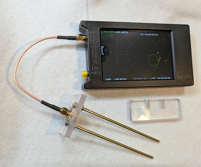
I was getting useful measurements with a 12-inch probe. But the issues listed above suggested a scaled down probe was at least worth a try. The "Tiny Probe" shown here is scaled to about 4-inches in length. Experiments have shown it to provide reliable data and mechanically it is easier to work with. I think it is worthy of adding to the toolkit, and thus this writeup.
Construction -
I used 0.25-inch thick polycarbonate (Lexan) for the mounting plate that holds the rods.
This is an OK but very adequate RF plastic for this use,
but a great mechanical plastic. The mechanical strength is a big plus and I recommend against using Plexiglass.
The rods go through a pair of 0.136" holes (or use 9/64"), separated by 0.75-inch.
The flange SMA connector is offset in position from the line through the two rods, by 0.50-inches.
This gives enough room so that the rod mounting and the SMA mounting do not interfere.
I milled into the mounting plate for the SMA such that the plastic is only 1/16-inch thick there.
As an alternative, a 1/16-inch thick side plate could hold the SMA and be fastened to the strong rod
holding plate.
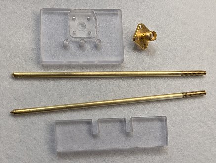
The lower piece of 0.25-inch thick polycarbonate is a spacer block that is used when starting the probe into the soil. It has the 0.75-inch spacing of the slots. The slots are made slightly wider than the rod diameter so that they do not bind. By being slotted, the spacer block can be removed after the probe is well into the soil.
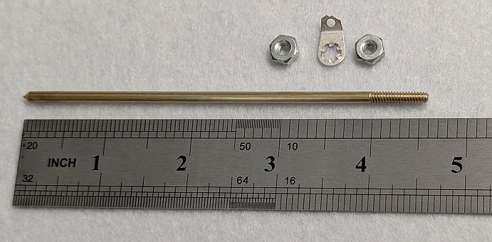
The rods are made from 1/8-inch brass stock. This is threaded with a 6-32 hand die over 0.6 inches of rod. The rod is cut to a total length of 4.6-inches and little tapers are ground/filed onto the un-threaded end of the rods. The mounting hardware is a pair of 6-32 x 5/16 nuts and a short solder lug.
Threaded rod is available that would simplify the construction. It may be a bad idea though, as the rod surface might interfere with smooth insertion. I have not tried that type of rod.
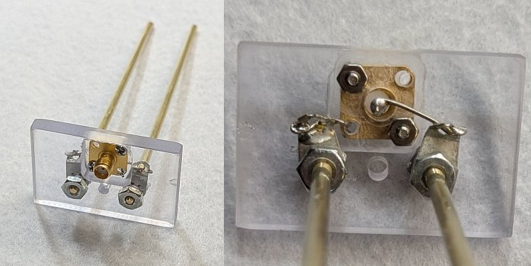
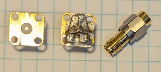
The ground connection starts with a #20 wire soldered to the SMA flange, on the threaded body side. The wire drops down through any of the mounting holes, as we only need two mounting screws. This is put on to the connector before the connector is put on the mounting plate. A second #20 wire wraps once around the SMA center pin. After mounting the SMA flange with a pair of 2-56 x 1/4-inch screws we are ready to add the two rods. As can be seen in the picture, there is a small solder lug on each rod. These lugs terminate the two #20 wires with no regard for polarity. Arrange for the wires to be short, but also avoid coming close to any surface that might short something out.
That is all there is to the construction.
Two more of the same SMA flange connectors were modified to be VNA calibration standards. This places the reference plane at the back surface of the SMA flange. The Open is simply the connector with the center pin filed flush with the flange. This does have a fringing capacity of 0.03 pF, but that is small enough to be ignored The Short used some scrap Solder-Wick to cover the back surface of the flange. Any length Load will work with this as there is no phase involved at the center of the Smith Chart.
Characterizing the Tiny Probe - [UPDATE: 7 March 2026 - Further experiments here and conversation with K6STI has shown it to be both practical and to give better accuracy to mount the nanoVNA to the Tiny Probe with a simple SMA male-male adapter. This raises the frequency of common-mode resonances. So far it has been practical to operate the "PAUSE" menu item while physically this close to the ground. An additional update is to leave the 0.25" thick plastic spacer at the SMA end of the probe, making measurements simpler and the probe more mechanically stable. This adds 0.15 pF of stray capacity that is accounted for in the "!Dimensions" line.]
For reference purposes, the parallel rods have a calculated characteristic impedance of 297 Ohms and the 4.3-inch length has a capacitance of 2.8 pF plus a small amount of fringing capacity. Additionally, the calculated total inductance of the various conductors that connect the two rods to the connector is 14.4 nH [Updated 7 Mar from 14.0]. If you follow the procedures for the gnd.exe program, it needs a measurement, in air, to trial-and-error estimate the stray capacity and the associated series resistance that will make the relative permittivity 1.0 and the low frequencies loss less. This works from the .s1p scattering parameter file that is measured in air. Following this routine we find a capacity of 1.85 pF [Updated 7 Mar from 1.77 pF] with a series resistance of 1 Ohm [Updated 7 Mar from 71, removal of ferrite bead with SMA adapter] is needed. By including this data as a line at the top of the .s1p file, it will automatically be included with the measurement data. These values do not change with different soil. The line is: !Dimensions 3.93 0.25 0.75 0.125 14.4i 1.85 1.0
Note that the 1.85 pF stray capacity includes the mounting plate, hardware and 0.25-in plastic spacer, but excludes the capacities between the two rods. Also, the air measurement will usually be done with a nanoVNA. This measurement tool is self powered and small allowing it to be un-grounded. This becomes a critical issue for soil measurements and will be discussed in the next section. But, for the air measurement, it is still best to keep probe close to VNA, have a VNA with built-in SD Card storage, and suspend the probe away from metallic objects, i.e., in air.
The values in the "!Dimensions" line probably provide a good starting point, but are best confirmed using your own hardware.
We expect that the lower frequency accuracy of this small probe is not going to be up to that of the 1 to 2 foot type. The place this shows up first is in measuring the probe while only in air. At frequencys in the lower MHz range, the probe must be a small value low loss capacitor. Using this model, I measured this Tiny probe as 3.25 pF (3.40 pF if the spacer plate is included). A larger probe (but not the biggest) with 12-inch long 1/4-inch rods spaced 2-1/2 inches was measured as 5.9 pF, so it would have about half the capacitive reactance. The issue here is that 3.25 pF at 1 MHz has a reactance of about 49K Ohms which is 1000 times the reference 50 Ohm resistance. It is a measurement that can acquire errors easily.
The capacity between the rods increases when placed into soil. We can calculate this capacity which in air is 2.8 pF for the Tiny Probe and 6.1 pF for the 12-inch probe. In soil, the capacity can increase greatly, primarily because of the polarized water molecules in the soil. This is the relative permittivity and might be 20, for which the capacities go up to 56 pF and 122 pF. This moves the reactance values into regions that are much easier to measure. Also, note that the difference in capacity of the probes is in the order of 2:1 which is less than the 3:1 length differences.
Measuring soil with the Tiny Probe - So, we have our Tiny Probe, what are we going to do with it? In short, the probe is small enough that we can identify a soil sample area out around our antenna, push the probe into that soil and measure it with a nanoVNA. Doing this over a number of spots and over the seasonal changes will give a picture of our local "RF ground." This writeup doesn't begin to addresss all the issues of antenna modelling, What we can do is to take a measurement to show how that is done.
[Updated 7 Mar:] The nanoVNA I am using is the "-H4" varient. This was chosen because it easily saves measurements to an SD card, and therefore does not require a grounded USB cable to be operated. This means the capacity between the VNA case and the nearby soil is minimized. The VNA is connected to the probe by a simple SMA male-male adapter. The goal is to minimize the interaction of the measuring instrument from the soil being measured. Along those lines, in the following measurement, it is critical that we do not touch the VNA, but rather use an insulated plastic item to run the touch screen.
To set up VNA, we need to go toward slow but accurate settings. The following need addressing (only the frequencies are saved with the Cal data. The others need entry every time the nanoVNA is powered up):
Careful calibration is needed at the probe end of the cable. Open, Short and Load are needed, but you can skip Isoln and Thru. If you save this calibration to one of the numbered pre-sets, it can be used to save time on future soil measurements. Just be sure to use the same RF cable setup every time.
It is time to go to the outside yard and measure some soil. Be sure you have an SD card pushed into the VNA (practice this step with the VNA turned off to see how it goes in---it is a bit tricky, at least on my VNA). Out in the yard, start with a surface patch that is clear down to bare soil. We are not measuring the lawn. Use your plastic spacer to get the rods started and push the probe into the soil. Push on the the probe to get the plastic spacer tighly secured between the mounting plate nuts and the ground. Connect on the SMA adapter and the VNA. You shoud see a simple Smith Chart trace, starting at the horizontal middle line and rotating smoothly in a clockwise direction as the frequency increases.
It seems practical to attach the nanoVNA, SMA adapter and Tiny Probe together and insert this entire group into the ground. BUT, be careful about nanoVNA damage. Push on the Tiny Probe. Do not push on the nanoVNA. And when removing the probe, do the same in reverse and always pull on the Tiny Probe mounting plate.
Stand back for at least 10 seconds and let a clean measurement procede. Tapping the screen to bring up menu items will show a "Pause Sweep" if you are at the top level screen. Hit Pause Sweep and you have frozen the measurement and you can touch anything. The thing to touch is "SD Card" followed by "Save S1P." You will either get an automatically assigned file name, or you can tap one in, including a final "Return" arrow. Congratulations! You have measured the soil.
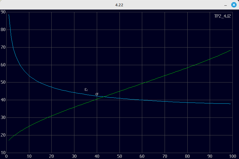
The simple ASCII text S1P file can be read by your PC. If you will be using multiple probes, it is a good idea to use any text editor to add the "!Dimensions" line shown above to the S1P file. If only one probe is used, gnd.exe will save the information, once it is set. Next, the K6STI gnd.exe program is used to reduce your new S1P file. Figure 6 shows a sample result from my back yard during the wet season. Notice the variation of permittivity and conductivity with frequency. If you study the information about the gnd.exe program, many subtleties will be seen. This is a good area to spend study time.
An un-tried idea is to dig a hole in order to get data, using the Tiny Probe. The hole might be 1 to 3-feet deep. If you can keep one edge of the hole shovel smooth, you should be able to push the probe into that surface horizontally. Doing this every 6-inches or so, going down into the hole, gives a vertical profile of the soil. The Tiny Probe is small enough that we can treat the sample as being uniform. If the soil is loose enough that it doesn't form a smooth surface, it may lead to some measurement errors. We do know that it is difficult to compact the soil as well as nature does, if we ever stir it up.
Getting back to your measurements, try measuring multiple spots and during different seasons. Every location is different and variations are seen. If you get bored with measuring the soil, try using the data to model your antenna farm. I think that is how we got here. Happy Measuring!
Acknowledgement - About six months ago, I came into this ground measurement deal not sure which end of the probe to put into the ground. Since then I have learned so much and have been able to characterize the ground in my area with reasonable confidence. This has been helped along in a big way by my mentors, K6STI and N6LF. Thanks, Brian and Rudy. And it is fun besides.
Issued 26 February 2026, revised 28 February 2026 - All Copyright © Robert Larkin 2026